Fatima - فاطمة

DIABETES PREDICTION

Predicting Diabetics in Pima Indians

In this project, we designed a supervised learning model for predicting whether a patient has diabetes or not.

Data Source

This dataset is originally from the National Institute of Diabetes and Digestive and Kidney Diseases and we used it from kaggle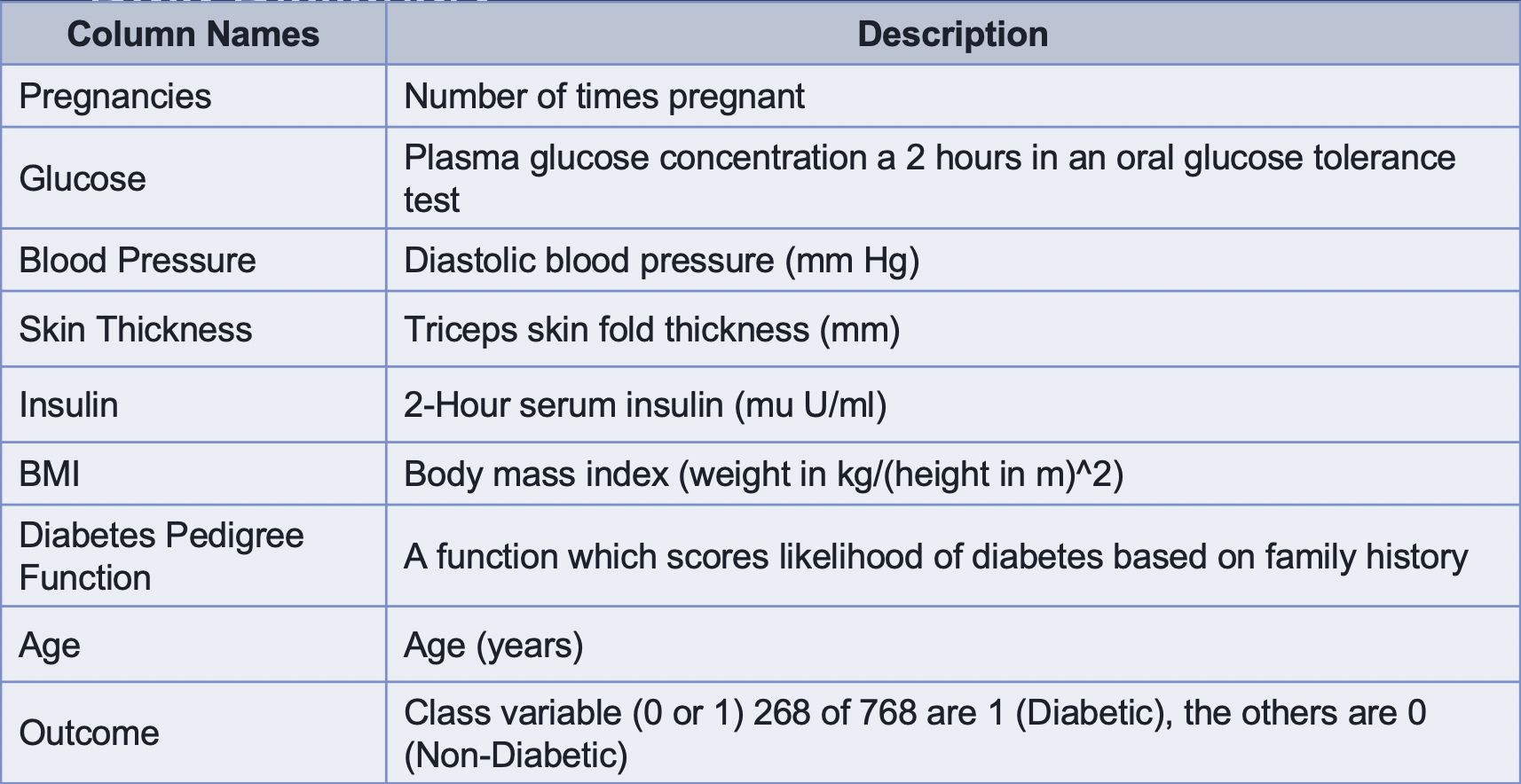

Data Insights

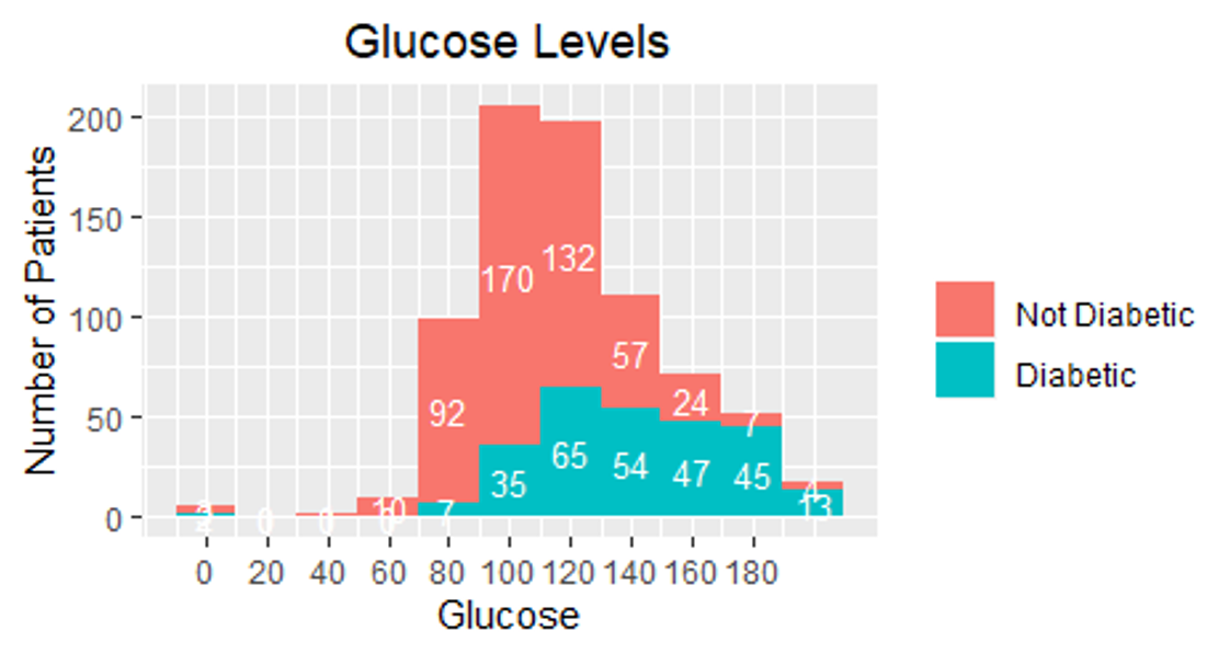
It was essential as a first step to pulling up some relationship between the columns in the dataset; the ratio for diabetic to non-diabetic is increasing after the age of 40. It was also increasing as the glucose level increase for the patients, which does make sense.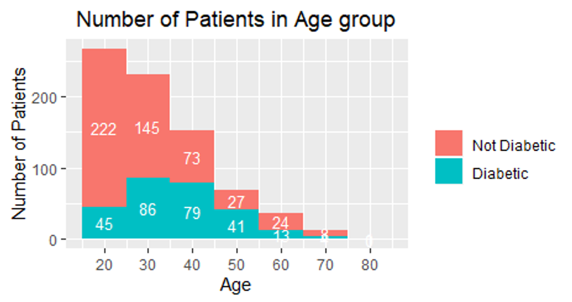

The correlation matrix and the heat map show that no two variables have a high correlation. The highest correlation is between Age and Pregnancies (0.54), which is not significant enough (>0.7) to be explored more.

Modeling

After that, we developed a model to predict if a patient has diabetes or not. For this, the first step would be to split the data into train and test data sets.

Logistic Regression Model We started with Logistic Regression. Logistic regression, also called a logit model, is used to model dichotomous outcome variables. In the logit model, the log odds of the outcome are modeled as a linear combination of the predictor variables. Logistic regression is conceptually similar to linear regression, where linear regression estimates the target variable. Instead of predicting values, as in the linear regression, logistic regression would estimate the odds of a particular event occurring. Logistic Regression is a supervised parametric learning model. In other words, the data should obey certain assumptions before developing the logistic regression model.
Assumptions of the Logistic Regression Model

Binary logistic regression requires the dependent variable to be binary, and ordinal logistic regression requires the dependent variable to be ordinal.
- Our dependent variable (Outcome) is a binary categorical variable.

Logistic regression requires observations to be independent of each other. In other words, the observations should not come from repeated measurements or matched data.
- Each row in the data set is independent of that of the other.

Logistic regression requires there to be little or no multicollinearity among the independent variables. This means that the independent variables should not be too highly correlated with each other.
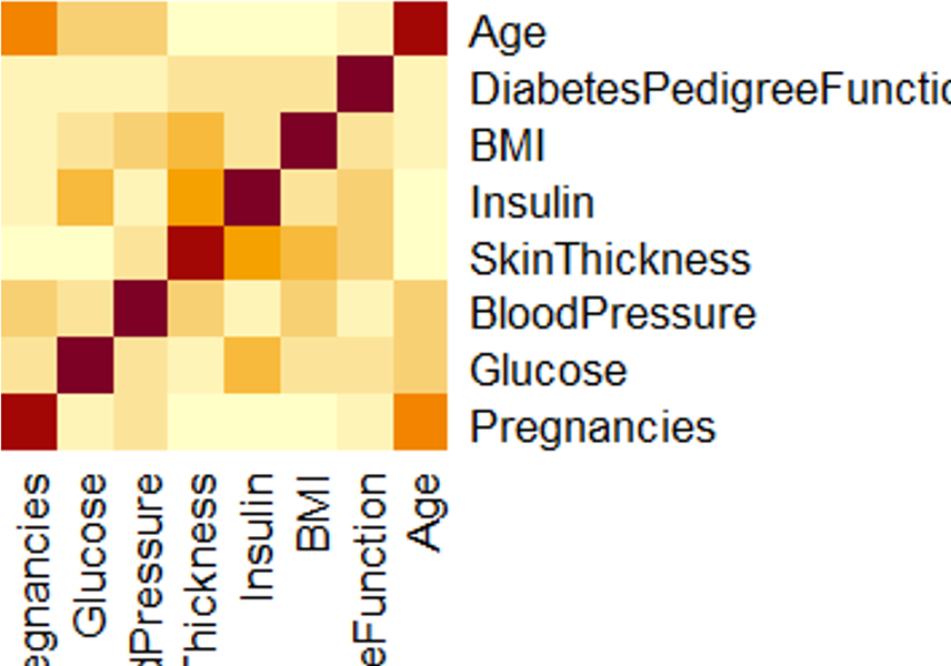
- From the correlation matrix, there is not much collinearity between the columns

Logistic regression assumes the linearity of independent variables and logs odds. Although this analysis does not require the dependent and independent variables to be related linearly, it requires that the independent variables are linearly related to the log odds.
- The independent variables are linear with log-odds.

Logistic regression typically requires a large sample size.
- In our data set, we have 798 observations, which are large enough for eight independent variables.

Building the Model

As all the assumptions are satisfied. we developed the model

Understanding the Results

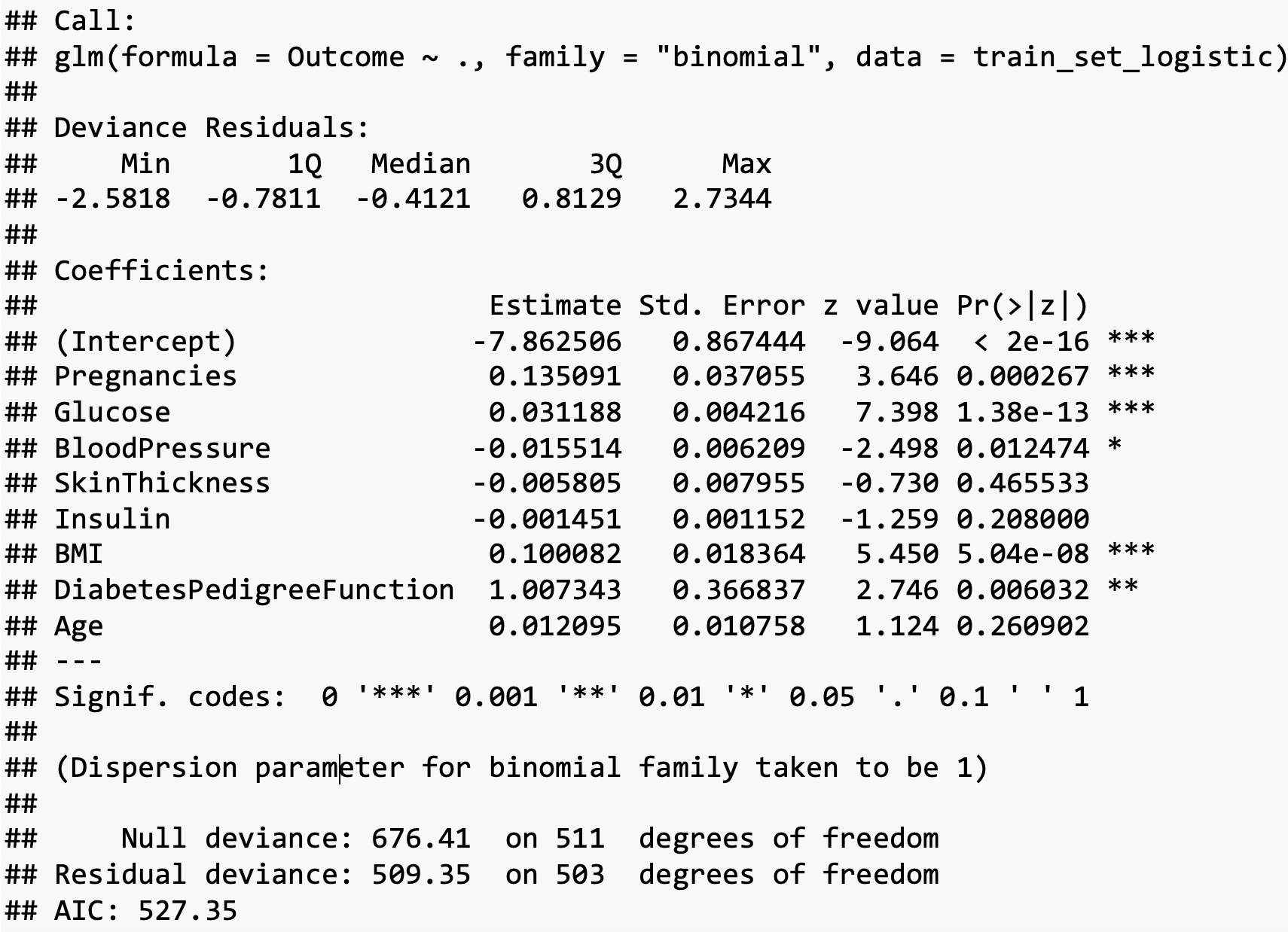
These were the results obtained for a logistic regression model. The result can be interpreted as follows:

Intercepts, Estimates, Standard Errors, and P values.

We have various columns and estimate values. The estimated values indicate the slope for the best fit line, and each column’s value is multiplied by this slope. Then we have the standard error of the slope for each variable in the model. We also have the z scores associated with each column. The last column is the p-value for these z scores. If the p-value falls below 0.05(95% interval, then those columns are highlighted using the asterisk (*) symbol). The first row consists of the intercept, which indicates the offset that has to be added to the model equation.

Null and Residual Deviance The null deviance shows how well the response variable is predicted by a model that includes only the intercept (grand mean). In contrast, residual deviance is the deviance with the inclusion of independent variables. Hence for calculating the null deviance, the degrees of freedom will be 512-1=511, and we have 503 degrees of freedom for residual deviance (503=512-8-1). We subtract eight, as we have eight independent variables. Residual is the difference between the actual and predicted value. So lower the residual score better than the model.

AIC Akaike’s Information Criterion (AIC) is -2log-likelihood+2k, where k is the number of estimated parameters. It is useful for comparing models of different models. Lower the AIC better is the performance of the model.

Fisher Scoring Iterations This is the number of iterations to fit the model. The logistic regression uses an iterative maximum likelihood algorithm to fit the data. The Fisher method is the same as fitting a model by iteratively re-weighting the least squares. It indicates the optimal number of iterations. Similar to Linear Regression, the model generates a linear equation using the given estimates and intercepts. Then the values from this equation will be converted into probabilities using the logit function. From the above result, we find that Pregnancies, Glucose, Blood Pressure, Diabetes Pedigree Function, MI, and Age are significant variables as they have the p values close to 0.05 or less than 0.05. The variable which does not contribute much for the model would be skin thickness.

Predicting in train and test data

After that, we tried to predict the values in the train and test set using our developed model.

The prediction column in both the data sets will now have probability values associated with each row. Now we need to convert this probability scores to whether a patient has diabetes or not using a threshold value.

Identifying the correct threshold value:

Before setting the threshold we took a look at the plot below: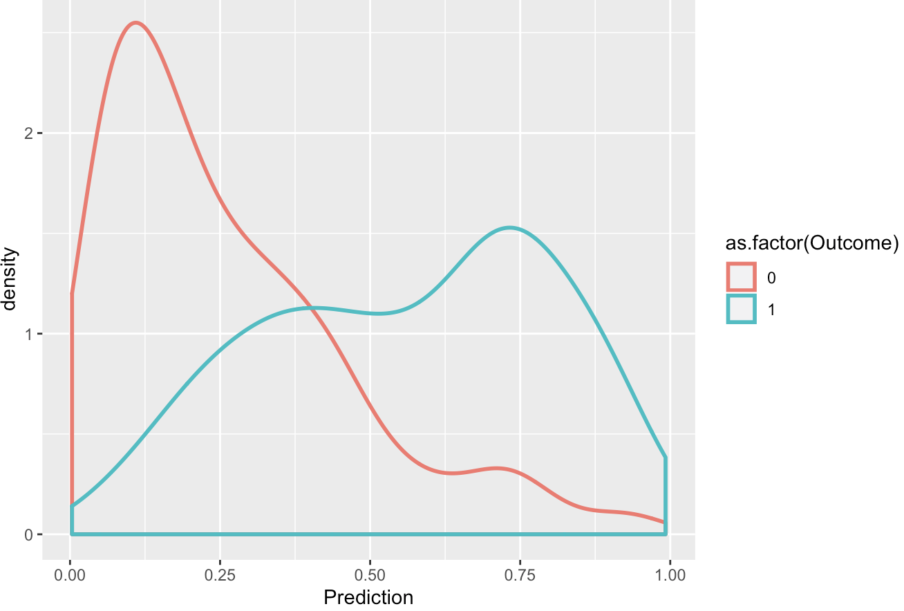

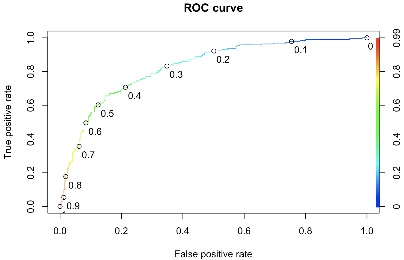
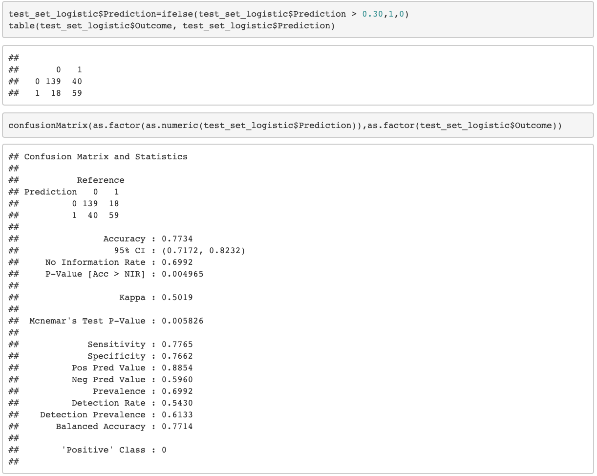
In an ideal situation, we would want the peaks of the two curves to be separated as much as possible. We also find that setting a threshold of 0.5 for the prediction score will not work out. From the graph, we find that the two curves cutoff at 0.3.
The other reason why a threshold of 0.5 will not work out is that, in our sample out of the 768 samples, only 268 are affected by diabetes. This is not a 50-50 proportion. In other words, the probability of encountering a diabetic patient is less than that of a non-diabetic patient. The (Receiver Operating Characteristics) ROC curve will now help us to fix the threshold.

We should choose the threshold value from this curve such that the ROC curve saturates and shows not much increase in True Positive Rate for a decrease in threshold value. So we will choose 0.30 to be our threshold value for our model.

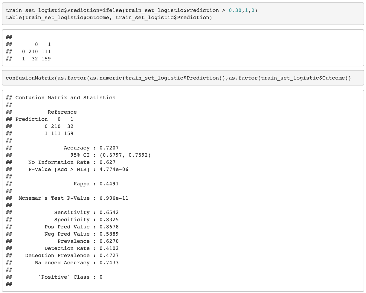
Confusion Matrix

For a threshold of 0.3, the model performs well and gives an accuracy of 75.2% on train data. Both sensitivity and specificity are also high.

The model performs similarly with the test data and has nearly the same accuracy, sensitivity, and specificity with that of the train data. This is a good indication that the model is not trying to overfit or underfit the data.

Decision Tree

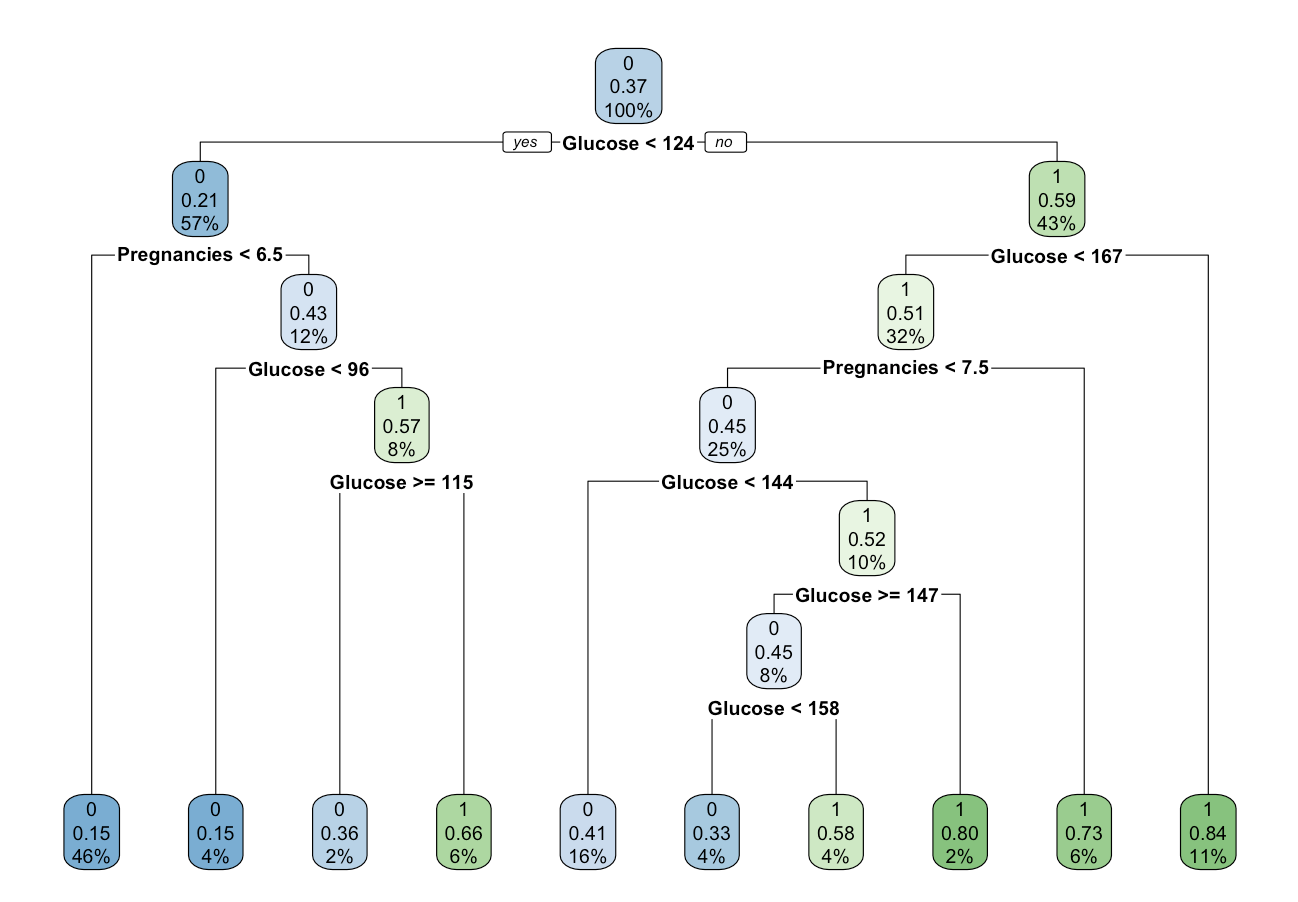
After that, we developed our next model, Decision Trees. Which are non-parametric models mean that they don't have any underlying assumptions about the distribution of data and errors.

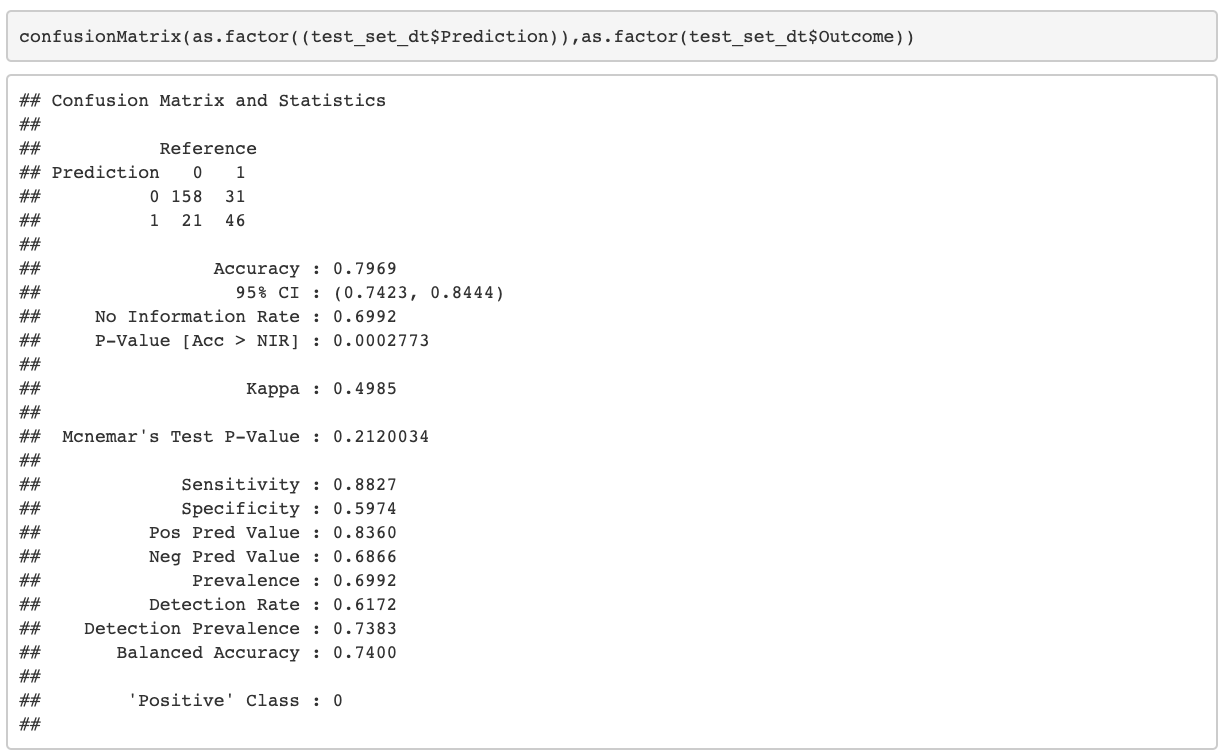
We were also able to plot the tree by selecting a very limited number of columns for better visualization. We can see the splits at each level and the number of elements considered at each level. This model is very easy to develop and understand.

Performance of the Model

The last step is analyzing the accuracy and other parameters of the decision tree model.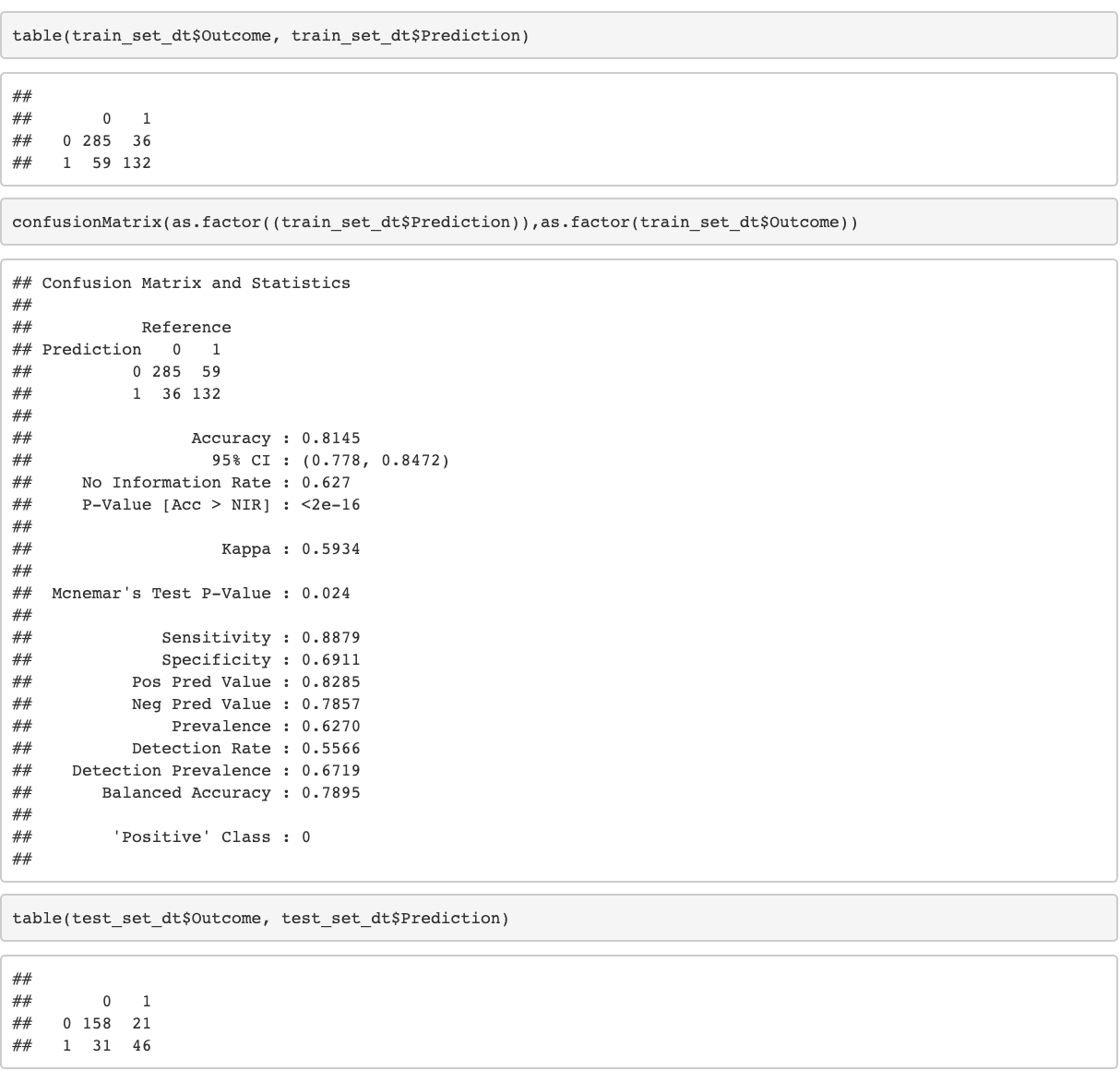

From the above result, we observe that the decision tree gives an accuracy of about 90% on train data and 70% on test data. This is because the decision tree has overfitted itself to the train data and hence the accuracy drops in test data. Even though the accuracy is less, the decision tree shows a very high sensitivity to test data.

Future Work

We can improve these models by adding extra features and fine-tuning them. For example, the logistic regression model can be improved by choosing a better threshold value. This can be done by evaluating a cost function for various threshold values. The decision tree model could have been pruned to avoid overfitting. Apart from these models, we could have tried other advanced models such as Ada Boosting trees, Gradient Boosting in Random forest, Deep Learning, and Neural Network models. We could also improve the training of all models by using k-fold cross-validation. One more option to improve the model would be to add more external features that can be related to diabetes in Pima Indians and we could also take a larger sample to improve the quality of our models.